PREDICTING SOIL PROPERTIES FROM HYPERSPECTRAL SATELLITE IMAGES

This project includes the soil parameter estimation algorithms based on various machine machine learning approaches, which have been developed for the purpose of participating the HYPERVIEW: Seeing Beyond the Visible Challenge

The members of the Team EagleEyes building this solution for the HYPERVIEW Challenge are:

Ridvan Salih Kuzu - Helmholtz AI consultant @ German Aerospace Center (DLR)
Frauke Albrecht - Helmholtz AI consultant @ German Climate Computing Centre (DKRZ)
Caroline Arnold - Helmholtz AI consultant @ German Climate Computing Centre (DKRZ)
Roshni Kamath - Helmholtz AI consultant @ Julich Supercomputing Centre (FZJ)
Kai Konen - Helmholtz AI consultant @ German Aerospace Center (DLR)

The submission file of the Team EagleEyes has improved upon the challange baseline by %21.9, with the first place on the public and private leader-boards. For the further details, please refer to:

[1] Kuzu, R. S., Albrecht, F., Arnold, C., Kamath, R., & Konen, K. (2022, October), Predicting Soil Properties from Hyperspectral Satellite Images, In 2022 IEEE International Conference on Image Processing (ICIP) (pp. 4296-4300). IEEE.

ICIP2022 Award Certificate

FOLDER STRUCTURE

The starter pack notebook provided by the Challenge Organization Committee is given under folder challenge_official_starter_pack.
The final submission of the Team Eagle Eyes is given under folder challenge_submission_eagleeyes.
The codes for Vision Transformer (ViT-L/14) based soil parameter estimation experiments are given under folder experimental_1.
The codes for Swin Transformer (Swin-T) and other DNN based soil parameter estimation experiments are given under folder experimental_2.
The codes for Random Forests and other classical machine learning based soil parameter estimation experiments are given under folder experimental_3.
The codes for PSE+LTAE based soil parameter estimation experiments are given under folder experimental_4.

INSTALLATION AND RUNNING

a. for Deep Learning based Approaches

If you want to run the project on docker containers, pull the customly built images for this project:

$ docker pull ridvansalih/clip:latest
$ docker pull ridvansalih/hyperview:latest

If you want to run the project on singularity containers, convert the docker images to singularity ones as described below:

$ export SINGULARITY_CACHEDIR=$(mktemp -d -p ${PWD})
$ export SINGULARITY_TMPDIR=$(mktemp -d -p ${PWD})
$ singularity pull clip_latest.sif docker://ridvansalih/clip:latest
$ singularity pull hyperview_latest.sif docker://hyperview:latest

After having the docker or singularity images, you can refer to the bash scripts (e.g. script_run_docker.sh, script_run_singular.sh) under the experiment folders in order to run them.

NOTE: Please be sure that you download the data and update the training and test folder paths in the bash scripts.

NOTE: Please be sure that the arguments given to main_hyper_view_training.py scripts in each experiment folder are valid for your hardware limitations.

b. for Classical Machine Learning based Approaches

Among classical machine learning approach, we have applied to Random Forests, Extreme Boosting and K-nearest Neighbor based regresssion algorithms. However, Random Forests algorith has outperformed the others, that is why our fine-tuning is based mostly on Random Forest as you can see the details in folder experimental_3. In order to run the Random Forests:

Use conda interactive: create environment from ai4eo_hyper.yml, activate environment ai4eo_hyper and run the script:

  $ conda env create -f ai4eo_hyper.yml
  $ conda activate ai4eo_hyper
  $ python3 r_train.py --in-data /2022-ai4eo_hyperview --submission-dir /ai4eo-hyperview/hyperview/submissions

Start a batch job:

  $ cd experimental_3/random_forest_b/jobs
  $ sbatch submit_trial.sh

Use Singularity & Docker:

  $ singularity pull docker://froukje/ai4eo-hyperview:rf
  $ sbatch submit_singularity_trial.sh

THE APPROACH

Abstract

The AI4EO Hyperview challenge seeks machine learning methods that predict agriculturally relevant soil parameters (K, Mg, P₂O₅, pH) from airborne hyperspectral images. We present a hybrid model fusing Random Forest and K-nearest neighbor regressors that exploit the average spectral reflectance, as well as derived features such as gradients, wavelet coefficients, and Fourier transforms. The solution is computationally lightweight and improves upon the challenge baseline by 21.9%, with the first place on the and private leaderboards. In addition, we discuss neural network architectures and potential future improvements.

Index Terms— hyperspectral images, random forests, artificial neural networks, soil parameter estimation, regression.

1. Introduction

Machine learning methods are employed widely in remote sensing [1]. In particular, agricultural monitoring via remote sensing draws significant attention for various purposes ranging from early forecasting of crop yield amount [2] to the estimation of soil composite [3].

Predicting the fertility indicators of soil, such as percentage of organic matter, or amount of fertilizer, is one of the leading research topics in earth observation [4] due to the emerging needs for improving the agricultural efficiency without harming nature. Particularly, the European Union Green Deal gives special importance to supporting conventional farming practices with earth observation (EO) and artificial intelligence (AI) for resilient production as well as healthy soil and biodiversity [5].

The AI4EO platform seeks to bridge the gap between the AI and EO communities [6]. In the AI4EO Hyperview challenge, the objective is to predict soil properties from hyperspectral satellite images, including potassium (K), magnesium (Mg), and phosphorus pentoxide (P₂O₅) content, and the pH value [7]. The winning solution of the challenge will be running on-board the Intuition-1 satellite.

In this manuscript, we present the solution to the AI4EO Hyperview challenge developed by Team EagleEyes. Section 2 discusses the hyperspectral image dataset, Section 3 covers feature engineering and experimental protocols for different learning strategies, and Section 4 presents the preliminary performance results for predicting the given four soil properties. Eventually, we conclude in Section 5 and give an outlook on future work.

2. Dataset

The hyperspectral images are taken from airborne measurements from an unspecified location in Poland. In total, 1732 patches are available for training, and 1154 patches remain for testing. Each patch contains 150 hyperspectral bands, spanning 462 − 492 nm with a spectral resolution of 3.2 nm [7].

Samples in the dataset have been segmented into patches according to the boundaries of the agricultural fields. As shown in Figure 1, the patch size distribution is skewed: About one third of the samples is composed of 11 × 11 px patches, and 60% of the patches are less than 50 px wide.

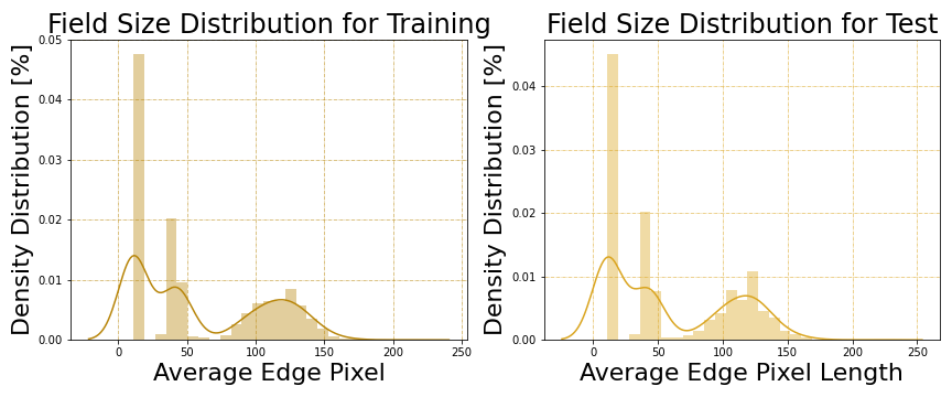
Figure 1: Distribution of dataset in terms of different patch sizes.

The training data provides ground truth for all four soil parameters. The target values for P₂O₅ lie in the range of [20.3−325], for K in [21.1−625], for Mg in [26.8−400], and for pH in [5.6−7.8]. As shown in Figure 2, for P₂O₅ and K, the target values follow a log-normal distribution with positive skewness, while the Mg and pH values are more Gaussian distributed. Besides, pH measurements are mostly clustered in the intervals of 0.1.

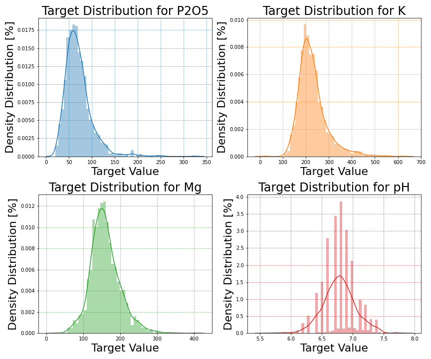
Figure 2: Distribution of target values for each soil parameter.

3. Experimental Framework

In this section, we present the feature engineering approaches, experimental protocols for different learning strategies and metrics utilized for validating our approach.

3.1. Data Processing and Augmentation

3.1.1. Feature engineering for traditional ML approaches

As mentioned in Section 2, the samples are 3-dimensional patches with dimension (w × h × c) where width (w), and height (h) have varying sizes, but channel (c) is fixed to represent 150 spectral bands.

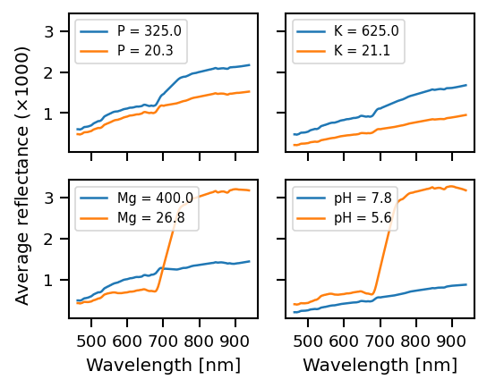
Figure 3: Comparison of average reflectance for different agricultural fields for each soil parameter.

Figure 3 shows the average reflectance as a function of wavelength for the samples with minimum and maximum value of the respective soil parameter. These average reflectance curves are remarkably dissimilar for different values of the target variable. Thus, we use the average reflectance as a base feature in our experiments, and derive additional features from it. The list of the features is as follows:

average reflectance, its 1^st, 2^nd and 3^rd order derivatives, ([1×150] dimension for each, [1×600] in total),
discrete wavelet transforms of average reflectance with Meyer wavelet [8]: 1^st, 2^nd, 3^rd, 4^th level approximation and detail coefficients ([1×300] dims. in total),
for each channel (c) of a field patch (P), singular value decomposition (SVD) has been conducted: P_(w×h) = UΣV^T, in which Σ is square diagonal of size [r×r] where r ≤ min{w, h}. The first 5 diagonal values (σ₁, σ₂, σ₃, σ₄, σ₅ ∈ Σ) from each channel are selected as features ([1×750] dims. in total),
the ratio of 1^st, 2^nd diagonals: σ₁/σ₂ ([1×150] dims.),
Fast Fourier transform (FFT) of average reflectance and FFT of σ₁/σ₂: real and imaginary parts are included ([1×600] dims. in total).

To sum up, for each field patch, a [1×2400] dimensional feature array is extracted. Some of those features for different agricultural fields are illustrated in Figure 4. For data augmentation, 1% random Gaussian noise is added to both input features and target values.

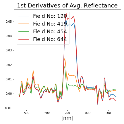
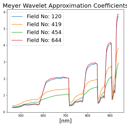
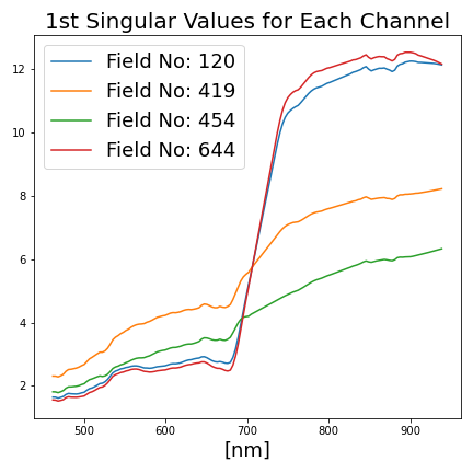
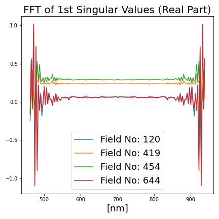
Figure 4: Selected additional features derived from the agricultural field patches.

3.1.2. Feature engineering for deep learning approaches

For experimenting on neural networks, either a raw patch, P_(w×h×c), or random patch subsets or pixel subsets from the raw patch is treated as a feature from a field. For data augmentation, we randomly add Gaussian noise, scale, crop, and rotate the field patches.

For both feature engineering approaches, we experimented with different data normalization techniques, including min-max scaling, standard scaling, and robust scaling.

3.2. Exploited Models

During development, classical machine learning approaches, such as Random Forest (RF), K-Nearest Neighbour (KNN) and eXtreme Gradient Boosting (XGBoost) regressors were investigated. Additionally, different neural network architectures were explored. Since the final solution is supposed to run on the Intuition-1 satellite, solutions that require low computational resources are of special interest.

3.2.1. Classical machine learning architectures

We used the RandomForestRegressor (RF) and KNeighborsRegressor (KNN) implemented in the scikit-learn package [9], as well as XGBoost [10] regressors. Since the latter does not support multiple-regression problems, the MultiOutputRegressor, also from the scikit-learn package, was wrapped around the XGBoost. For all model types, hyperparameter tuning was conducted using Optuna [11] with Bayesian optimization. However, we found the default parameters performed best and only changed the number of estimators to 1000. For all of our experiments, RFs perform better than the XGBoost and KNN algorithms.

3.2.2. Deep Neural networks

We experimented with various neural network architectures, including Transformers [12] [13], MobileNets [14], CapsuleNets [15], multilayer perceptrons, as well as autoencoder architectures [16] and attention networks, such as PSE+LTAE [17]. To exploit the pretrained weights of the networks, we experimented with several input modalities:

channel-wise dimensional reduction from (w × h × 150) to (w × h × 3) via convolution operation and later feeding the samples into the pre-trained models;
dropping the input layers of the pretrained networks mentioned above, and attaching our custom input layers that accept (w × h × 150) dimensional samples;
feeding each channel (w × h × 1) of a sample into the 150 parallel and weight-sharing pretrained networks;
expanding the input dimension as (w × h × 150 × 1) to exploit 3D neural networks such as CapsuleNets ;
flattening the input dimensions, or subsampling the input for exploiting 1D neural networks such as multilayer perceptrons or autoencoders.

Nonetheless, many of those trials performed worse than the RF, except for the Transformers with the pretrained weights (ImageNet-21k for Swin-T and CLIP for ViT-L/14 ), when the channel-wise dimensional reduction operation was attached to it as an input layer.

For designing those experiments, we used the Keras framework with Tensorflow version 2.8.0 [18] and the Pytorch framework version 1.10.0 [19].

3.3. Evaluation Metrics

The evaluation metric takes into account the improvement upon the baseline of predicting the average of each soil parameter (MSE_bl). For a given algorithm, it is calculated as:

$$\mathrm{Score} = \frac 1 4 \sum\limits_{i=1}^{4} \frac{\mathrm{MSE_{algo}}^{(i)}}{\mathrm{MSE_{bl}}^{(i)}}, \,\, \textrm{ where:}$$

$$\mathrm{MSE_{algo}}^{(i)} = \frac 1 N \sum \limits_{j=1}^N (p_j^{(i)} - \hat p_j ^{(i)})^2 .$$

4. Results and Discussion

Among our experiments listed in Section 3.2, the best performing ones on the public leaderboard of the challenge are:

RF regression, by achieving 0.79476
Swin Transformer (Swin-T), by achieving 0.80028
Vision Transformer (ViT-L/14), by achieving 0.78799

The models show comparable performance, however, the RF is computationally more lightweight. Since this would be advantageous for running the model on the target Intuition-1 satellite, we selected the RF for further optimization.

As summarized in Table 1, the average of 5-fold cross validation on the training set with RF yields a validation score of 0.811. Note that while we improve on the baseline for all four soil parameters, the performance varies. Mg is predicted best (0.734), and P₂O₅ is predicted worst (0.874).

Table 1: Cross validation with RF (the lower score is better).

Field Edge (pixel)	# of Fields	P2O5	K	Mg	pH	Average
0-11	650	1.050	1.008	1.019	0.866	0.985
11-40	94	0.491	0.581	0.539	0.981	0.648
40-50	326	0.724	0.754	0.416	0.777	0.668
50-100	138	0.683	0.660	0.618	0.749	0.677
100-110	113	0.911	0.591	0.398	0.764	0.665
110-120	118	0.883	0.812	0.614	0.731	0.760
120-130	132	0.895	0.776	0.644	0.656	0.742
130+	161	0.808	0.761	0.842	0.790	0.801
Entire Fields	1732	0.874	0.828	0.734	0.807	0.811
Public Leaderboard Score on the Test Set		0.79476

For the RF regression, the feature importance can be determined. Figure 5 shows the derivatives of the average spectral reflectance contribute the most, followed by the features derived from SVD and FFT. Figure 6 shows the importance of the spectral bands. The bands in the 650 − 670 nm, and those exceeding 850 nm are considered to be most important.

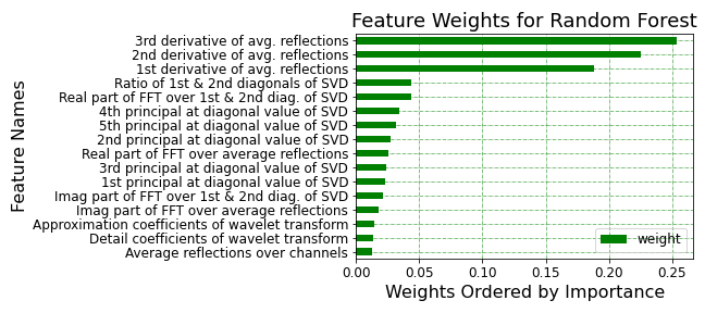
Figure 5: Feature importance weights for RF regressor.

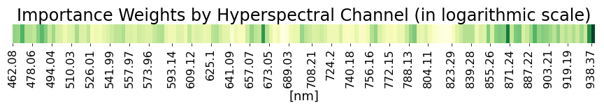
Figure 6: Hyperspectral band importances for RF regressor.

In order to analyze if the data skewness affects performance, the prediction scores are reported for different patch sizes in Table 1. Thus, we observe that the smaller patches ( ≤ 11 × 11 px) are the major source of the prediction error. This might stem from the higher variations in channel-aggregation due to a lower number of pixels. For mitigating this error source, alternative hyperparameter spaces and ML architectures were sought for smaller field patches. KNN regression with k ≥ 35 improved performance on the smaller patches (from 0.985 to 0.915) but, on the other hand, it performs worse than RF on larger patches.

Table 2: Cross validation with hybrid regressor (RF + KNN).

Field Edge (pixel)	Model	P2O5	K	Mg	pH	Average
0-11	KNN	1.002	0.953	0.993	0.710	0.915
11+	RF	0.766	0.720	0.564	0.772	0.706
Entire Fields	Hybrid	0.855	0.807	0.725	0.749	0.793
Public Leaderboard Score on the Test Set		0.78113

Therefore, a hybrid soil paramater estimator is proposed, combining KNN and RF regressors. Table 2 summarizes the performance of the hybrid model in which KNN predicts the soil parameters for smaller fields (mean edge length ≤ 11 px), while RF makes predictions for larger fields (mean edge length > 11 px). Thus, cross-validation performance on training set has been improved from 0.811 to 0.793. With this hybrid model, our team has preserved the top position in the public leaderboard by outperforming our former RF regressor (from 0.79476 to 0.78113).

Figure 7 shows density plots of the true vs the predicted soil parameters for the validation set. For all target variables, average values are predicted close to the 1 : 1 line, while extreme values are hard to estimate correctly.

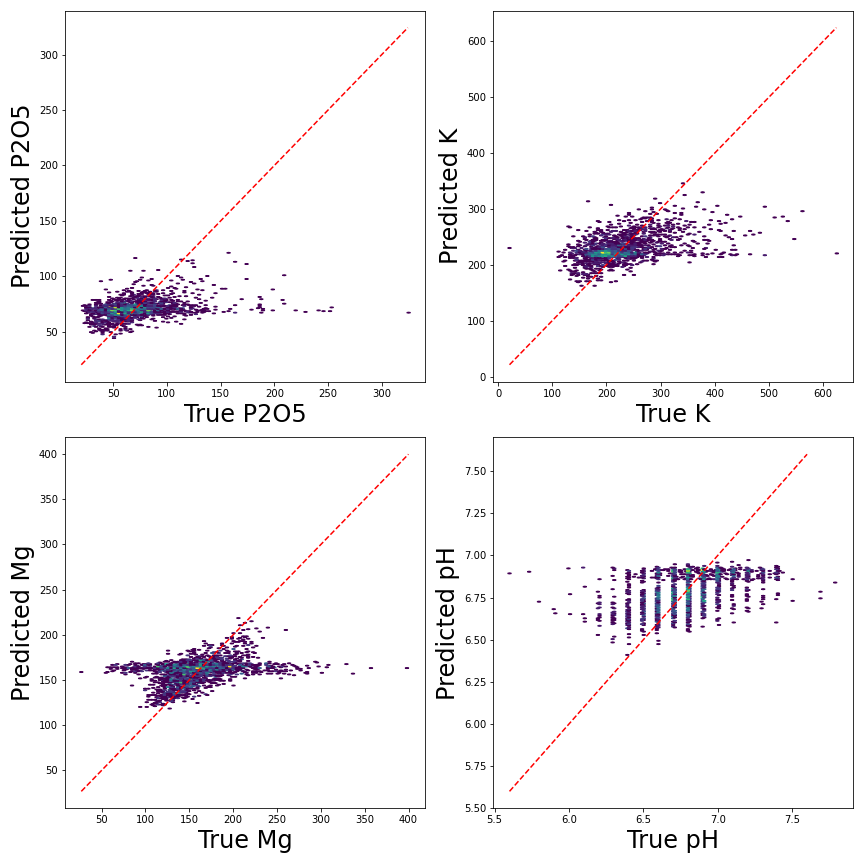
Figure 7: Ground-truths vs predicted soil parameters.

5. Conclusion and Future Work

In this paper, we demonstrated our solution to the AI4EO Hyperview challenge which seeks for the most efficient approach to predict soil parameters (K, Mg, P₂O₅, pH). With comprehensive feature engineering, and by building a hybrid solution based on the fusion of KNN and RF regression models, we achieved 21.9% improvement compared to the baseline, and preserved the leadership so far. In the future, we will select features and train models individually for the four soil parameters to optimize performance. Besides, we will conduct further experiments with novel architectures tailored to the provided challenge dataset.

Acknowledgments

We thank Lichao Mou for helpful discussions. This work was supported by the Helmholtz Association’s Initiative and Networking Fund through Helmholtz AI [grant number: ZT-I-PF-5-01] and on the HAICORE@FZJ partition.

Citation

In order to cite this study:

@INPROCEEDINGS{9897254,
  author={Kuzu, Rıdvan Salih and Albrecht, Frauke and Arnold, Caroline and Kamath, Roshni and Konen, Kai},
  booktitle={2022 IEEE International Conference on Image Processing (ICIP)}, 
  title={Predicting Soil Properties from Hyperspectral Satellite Images}, 
  year={2022},
  volume={},
  number={},
  pages={4296-4300},
  doi={10.1109/ICIP46576.2022.9897254}}
  